Talairach realignment warps an individual brain to a standard. Ideally, this allows one to identify anatomical structures based on their absolute Talairach coordinates. However, it warps the brain into a rather unnatural flattened shape and the accuracy of the results is always worth calling into question. All examples are for the tutorial. Download study1_norm+orig.BRIK and HEAD and brain+orig.BRIK and HEAD from the analysis directory. Download brain3d_cent+orig.BRIK and HEAD from the finished directory. Note that if you want to play with the talairached files, brain3d+tlrc is available in the finished directory. You should end up with these 6 files to practice talairaching:

• study1_norm+orig.BRIK and .HEAD,
• brain+orig.BRIK and .HEAD,
• brain3d_cent+orig.BRIK and .HEAD (the centered/aligned version)

Begin with a 3d volume that has been preprocessed and centered. Go to the directory containing that file and start afni:

> afni

This opens the afni graphical user interface (GUI):

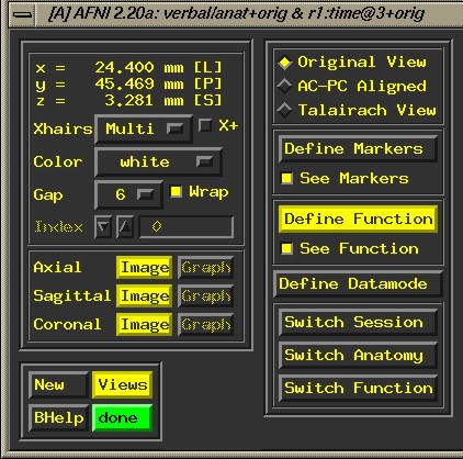
Choose "Switch Anatomy" from the lower right corner, and select the 3d volume that you wish to work with (choose "Set" to select volume and close the popup menu).
On the left (middle box), you should select all three different views to assist you in identifying the Talairach anchor points:

• Axial "Image"
• Sagittal "Image"
• Coronal "Image"

Additionally:

• Make sure "Original View" is selected in the upper right
• Select "Define Markers" and the gui will be extended on the right.
• Select "Allow Edits" from the extended menu to the right so you can pick the first set of anchor points for AC-PC alignment.

• Consult the following website for more advice: http://afni.nimh.nih.gov/afni/
• Next you must locate the following anchor points on the 3D brain image. Once you have located an anchor point and placed your cross hairs on it, select "Set" and go on to the next one. It is preferable to locate points on the same plane, though it is not always possible.
• Superior Edge of Anterior Commisure: Click "AC superior edge". Move up through the axials until you can't see the AC anymore. Then go down one slice to where you can see it. This is the superior edge. Click "set". In our tutorial data, the superior edge of the AC is located on axial slice 122, coronal slice 113, sagittal slice 61; x=4.950 mm L, y=-18.160 mm A, z=-5.571 mm I.
• Posterior Margin of Anterior Commisure: Relying on the axial view, find the image in which the AC is thickest. Find the back side of the AC on this image. This is the posterior edge. In our tutorial data, the posterior margin of the AC is located on
  axial slice 120, coronal slice 115, sagittal slice 61;
  (x=4.950 mm L, y=-16.207 mm A, z=-7.524 mm I).
• Inferior Edge of the Posterior Commisure: The PC is usually more difficult to see than the AC. Using the axials and coronals, find the line of white matter crossing between the two hemispheres above the colliculi. Open the sagittal image to make sure you can get the anterior and posterior commisures in the same sagittal plane. For our tutorial data,
  axial slice 113, coronal slice 140, sagittal slice 61;
  x=4.950, y=8.207, z=-14.360.
• Two Midsagittal Points: Using the midsagittal image (the sagittal image that opens by default in afni), try to find two points in the midcortical region, preferably in the same plane as the AC and PC anchor points (which are marked with little green squares as soon as you select "set" for each anchor point). From the AC, fan out to a position anterior and superior for the first point. From the PC, fan out to a position posterior and superior for the second point.
• Select "Quality Report". If you have done well, both angular measures in the quality report will be less than 4%. If you have not done well, you can go back to your anchor points and selectively clear each one and try again. Keep trying until you get a good quality report.
• Transform Data. After a good quality report, select "Transform Data".

• Now select "AC-PC Aligned".
• Select "Define Markers".
• When the "Define Markers" interface is displayed, select, "Allow Edits"
• Again, make sure all three views of the brain are open.
• You want to find cortex (choose views with whiter cortex not greyer meninges dispayed).
• You will see a new set of anchor points to identify and set:
  • Most Anterior Point: Use all three views to help find the most forward point in the cortex. In our tutorial data, this is on:
    axial slice 79, coronal slice 22 and sagittal slice 107
    (x=-12.000 mm R, y=-73.000 mm A, z= 9.000 mm S).
  • Most Posterior Point: Use the coronal view to help find this. In our tutorial data, this is on:
    axial slice 66, coronal slice 197 and sagittal slice 85
    (x=10.000 mm L, y=102.000 mm P, z= -4.000 mm I).
  • Most Superior Point: Use the axial view to help find this. In our tutorial data, this is on:
    axial slice 144, coronal slice 118 and sagittal slice 90
    (x=5.000 mm L, y=23.000 mm P, z= 74.000 mm S).
  • Most Inferior Point: Use the coronal view to help find this. Ignore the cerebellum. This point will be the bottom edge of a temporal lobe. In our tutorial data, this is on:
    axial slice 32, coronal slice 110 and sagittal slice 149
    (x=-54.000 mm R, y=15.000 mm P, z= -38.000 mm I).
  • Most Left Point: This is actually the rightmost side of the image. In our tutorial data, this is on:
    axial slice 67, coronal slice 138 and sagittal slice 31
    (x=64.000 mm L, y=43.000 mm P, z= -3.000 mm I).
  • Most Right Point: This is actually the leftmost side of the image. In our tutorial data, this is on:
    axial slice 101, coronal slice 124 and sagittal slice 164
    (x=-69.000 mm R, y=29.000 mm P, z= 31.000 mm S).
• When you have finished, run the "Quality Report". If there are too many errors, afni will not let you continue and you will need to clear suspect anchor points and try again.
• When the data is satisfactory, select "Transform Data". This creates a tlrc HEAD file.

• Now select "Talairach View".
• Select "Define Datamode".
• On the Define Datamode interface, select "Warp Anat on Demend"
• Also select: Anat resam mode "Li" (Linear anatomical resampling)
• Select: Write "Anat". This will create a BRIK file with the same name as your original 3d volume, but it will replace the "orig" extension with "tlrc". You will only see this additional extension if you look at a listing of your files in the shell. Afni will not display a file with this extension in its popup menus. Rather, it will allow you to select the original file AND "Talairach View" to display the 3d volume with Talairach coordinates.

• *You may need to close and reopen afni so that it can refresh its information about available files. Afni seems to have real difficulties with refreshing.
• At the command line:
  >adwarp -apar anat+tlrc -dpar func+orig
  will write out the dataset func+tlrc. Substitute the names of appropriate anatomical and functional datasets. You should also be able to choose "Define Datamode" in the gui, and then Write Many from the lower right panel.
• Select one or more functional image briks from the popup menus (these already should be preprocessed, centered and analyzed) and warp these into Talairach views as well.
• After you create the functional warping, you can select "Switch Function" to view a functional image overlaid on the anatomy (As long as you have selected "Warp function on demend"). Note that by choosing the 3D volume in Talairach View, you are, in effect, 'demanding' that the functional image be warped to it.

  ---

You will find that your talairached files are larger than the originals, and that they are resliced into 1 mm isotropic voxels (this is what makes them bigger). You will also find that all talairached files are the same size as each other (because they all have the same voxel size).

Skull Stripping

Once you have talairached the high resolution images, you can strip off the skull:
3dIntacranial -prefix output -anat input

>3dIntracranial -prefix brain_stripped -anat brain+tlrc

You can apply skull stripping to either the 2D or 3D high resolution talairached images (e.g., brain or brain3d). After brain stripping, you might want to go to Define Datamodes->Plugins->Render. Render will allow you to see a volume rendering of the head. You can try it on both the stripped and unstripped head. The render plugin will allow you to create a movie frame by frame.

For more interesting things you can do with a talairached image, see information on the built in talairach atlas and masking.