|
All
examples are for the tutorial. Download
the files from the analysis directory and unzip them to proceed:
- study1_norm+orig.BRIK
and .HEAD,
- block80.1D,
- brain+orig.BRIK
and .HEAD,
- optionally
brain3d+orig.BRIK and .HEAD
If
you wish to prepare images for presentation, there are some extra
issues to consider and this is the stage (prior to analysis) at
which you should do it. See the page on making Pretty
Images. If you are just doing the tutorial, you might want to
leave this till later.
Analysis:
Phase 1
In
this phase you apply the waver file to your
data to see which areas of activation are correlated to the conditions
defined by hemodynamic responses in that waver file.
Put
the above files into an analysis directory and cd to it. Type:
>afni
(or, after afni is open, choose Define Data Mode and Read Sess to
set up multiple sessions).
- A
'widget' window (GUI) will appear:
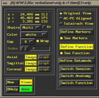
- Switch
Anatomy. A drop down window appears. Choose an appropriate *_norm
file (functional epan file). Click it to highlight it, else you
will not be able to access the graph. "Image" will show
you a picture of the data.
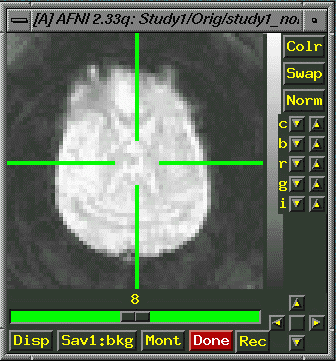
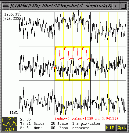
- "Graph"
will show you intensity values over time associated with each
voxel (The one in the yellow box in the center is the one your
green crosshairs point at.)
- At
the bottom right of the graph window, choose FIM => Pick Ideal
=>Choose and set the appropriate *.1D file. (Note: After you
pick the ideal, it will appear on the graph as a separate line
and have values for all points along the x-axis)
- FIM
=> Compute FIM =>fico (watch green progress meter)
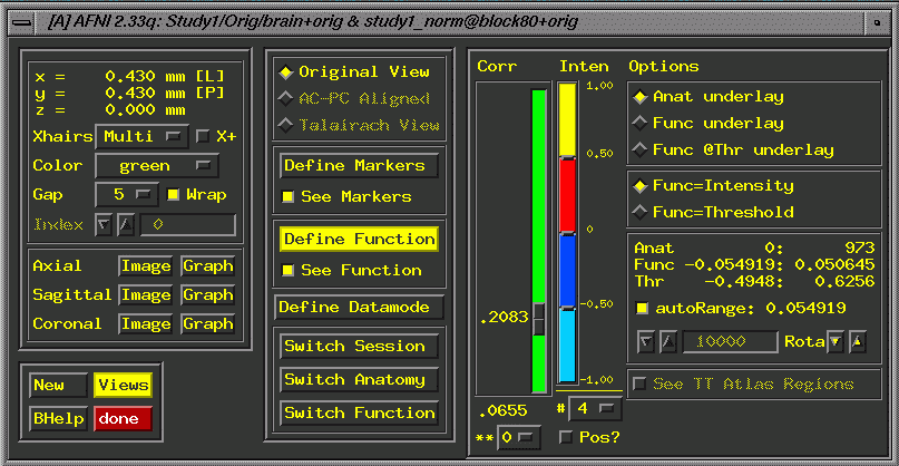
- Define
Function. This brings up additional widgets, a correlation bar
and color bar. Select 4 colors, change orange to red and set
the color change. If you leave the correlation slider at r=.5000,
you'll rarely see activation, so check to make sure you have
lowered it.
- Rename
first analysis: Define Data Mode=>Plugins=>Dataset Rename.
-Your
analysis will likely be at the bottom of the list with a prefix
like study1_norm@1. Change the number to the ideal name (e.g.
study1_norm@block80). Run and Close.
Cluster
Analysis: Part 2
- Define
Function=>choose p value (under correlation slider). Record
p and r.
- This
simply alters which functional activations will be visible. If
this is a second clustering, recheck Switch Function to make sure
it is using the correct dataset.
- Define
Data Mode =>Plugins=>3D Cluster
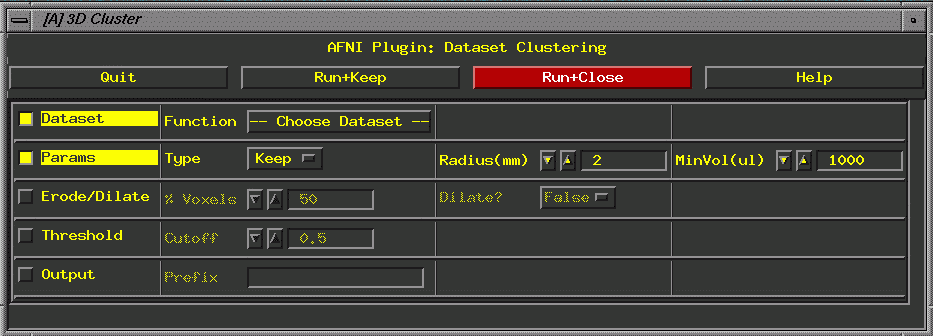
Dataset: file from first analysis (e.g., study1_norm@block80).
Radius: 3.8
Min vol: 150
Threshold: the r value from the correlation slider (double
check it).
Output: Condition_ideal_norm_pvalue_minvol (e.g., study1_block80_norm_p05_150ul)
Run and Close
Optional: Switch Anatomy, Select brain anatomy for pretty
overlay.
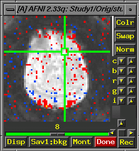
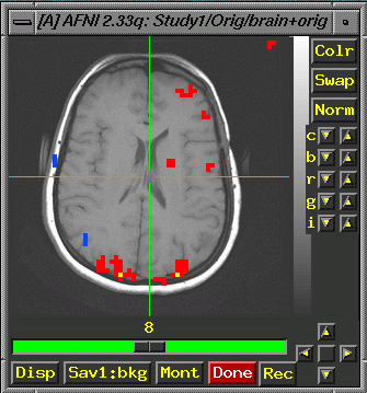
- You
now have a clustered fico BRIK
- If
you want it to display like the image below, choose "Switch
Anatomy" and select "brain" from the list.
- Then
choose "switch function" and select your study1_block80_norm_p05_150ul.
As long as "see function" is also selected, you should
now see an image like the one below:
After
looking at your initial output, you may want to fiddle with clustering
parameters to enhance images for presentation. To learn more about
pretty images, go here.
|